Route Optimization: How to Measure Fuel and Time Savings in Distribution
What is Route Optimization?

Finding the most efficient path under dozens of constraints at once is a far more mathematical job than it looks.
Route optimization is the mathematical and algorithmic approach to reaching multiple delivery points in the most efficient order. Trace it back to its academic roots and you land on classic operations research problems like the Travelling Salesman Problem and the Vehicle Routing Problem. On the ground, though, it is simply the thing that decides how your daily distribution plan turns out.
The optimization process considers the following variables:
- Distance and time: Physical distance between points and estimated driving time.
- Vehicle capacity: Weight, volume, and pallet limitations.
- Time windows: Delivery intervals specified by the customer.
- Driver constraints: Working hours, break requirements, and certifications.
- Traffic conditions: Historical and real-time congestion data.
- Vehicle specifications: Fuel consumption, emission class, and refrigeration capacity.
Optimization Goals
Route optimization is not a one-dimensional problem. Whatever your priority is, your objective shifts to match it:
- Distance minimization: Reducing total kilometers traveled.
- Time minimization: Shortening total operational time.
- Cost minimization: Lowering fuel, labor, and vehicle expenses.
- Capacity maximization: Increasing vehicle utilization rates.
- Service level: Improving on-time delivery rates.
Manual Planning vs. Algorithmic Optimization
Traditional manual planning, whether on paper or in Excel, runs into some hard limits:
- The human brain cannot optimize more than 15-20 points in its head.
- Weighing every variable at the same time is simply not possible.
- Even an experienced planner drifts 15-25% off the optimal solution.
- Reacting quickly to changes during the day is difficult.
Algorithmic optimization sits on the other side of that:
- Evaluates thousands of points in seconds.
- Accounts for all constraints simultaneously.
- Produces consistent and repeatable results.
- Rebuilds the route on the spot when conditions change.
The Optimization Paradox
The shortest distance is not always the most efficient route. Once traffic density, road quality, fuel consumption, and time windows enter the picture, a longer but faster or more economical route often wins. Real optimization is about balancing objectives that pull against each other.
VRP Algorithms and Solution Approaches
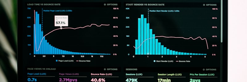
The Vehicle Routing Problem is one of the most heavily studied topics in combinatorial optimization.
Dantzig and Ramser first defined the Vehicle Routing Problem (VRP) in 1959, and thousands of academic studies have piled up on it since. It sits in the NP-hard class, which means that as the number of points grows, finding the optimal solution gets exponentially harder. The gap between a 20-point problem and a 200-point one is much wider than it seems.
VRP Variants
The basic VRP branches into different types depending on the constraints layered on top of it:
CVRP – Capacitated VRP
Each vehicle has a specific capacity limit. This is the most common variant and covers the bulk of distribution scenarios.
VRPTW – VRP with Time Windows
Each customer has a delivery time window they will accept. This is the variant that decides everything in last-mile delivery.
VRPPD – VRP with Pickup and Delivery
Scenarios that involve both delivery and collection. This is where reverse logistics and mixed operations come in.
MDVRP – Multi-Depot VRP
Distribution from multiple depots. Relevant for large-scale distribution networks.
DVRP – Dynamic VRP
Adaptation to real-time changes, such as new orders, cancellations, and traffic updates.
Solution Algorithms
1. Exact Algorithms
These guarantee the optimal solution but only work on small problems:
- Branch and Bound: Optimal solution via systematic search.
- Branch and Cut: An improved version using cutting planes.
- Mixed-Integer Programming: A mathematical programming approach.
Limitation: Calculation time becomes unacceptable beyond 50-100 points.
2. Constructive Heuristics
These build the route step by step, starting from an empty solution:
- Nearest Neighbor: Select the closest point at each step.
- Savings Algorithm (Clarke-Wright): Save by merging routes.
- Sweep Algorithm: Clustering via angular scanning.
- Insertion Heuristics: Add points to the most suitable position.
Advantage: Fast, easy to follow, and gives a solid starting solution.
3. Improvement Heuristics
These take the existing solution and refine it pass after pass:
- 2-opt: Swapping two edges within a route.
- 3-opt: Swapping three edges for more comprehensive improvement.
- Or-opt: Moving points or sequences.
- Relocate/Exchange: Transferring points between routes.
4. Metaheuristics
More sophisticated methods built for genuinely complex problems:
- Genetic Algorithms: Mimicking natural selection and mutation.
- Simulated Annealing: A method inspired by the metal cooling process.
- Tabu Search: Search with memory to escape local optima.
- Ant Colony Optimization: Simulating ant colony behavior.
- Particle Swarm Optimization: Optimization based on swarm intelligence.
Hybrid Approaches
In practice, most commercial optimization software does not stick to a single method; it blends them:
- Fast initial solution with constructive heuristics.
- Local improvement with improvement heuristics.
- Global search with metaheuristics.
- Multi-solution discovery via parallel computing.
Algorithm Selection
The right algorithm depends on the scale of the problem and the time you have. Under 50 points, you can try an exact algorithm. Between 50 and 500 points, hybrid heuristics give the best result. Past 500 points, metaheuristics and parallel computing become mandatory. And in real-time scenarios, speed usually comes before quality, because nobody can sit and wait minutes for a calculation.
Last-Mile Delivery Optimization

The shortest link in the chain, the last mile, is also the most expensive and the biggest headache.
Last-mile delivery is the stage where the product leaves the distribution center and reaches the end consumer’s door. It is the shortest segment of the chain, yet it swallows 40-50% of the total delivery cost. So it is the first place anyone serious about cutting costs should be looking.
Challenges of Last-Mile
Density and Distribution
High address density in urban delivery looks like an advantage at first glance, but the picture changes once you are out there:
- Finding parking eats into time.
- Waiting for elevators or climbing stairs stretches the clock.
- Traffic congestion creates delays you cannot predict.
- One-way streets and restricted zones lengthen the route.
Time Window Pressure
Consumer expectations narrow a little more every year:
- Same-day delivery is becoming the norm.
- Two-hour delivery windows are being requested.
- Real-time tracking and an ETA are no longer a hope but an assumption.
- Flexible delivery options (leave at door, give to neighbor).
Cost of Failed Delivery
The moment the recipient cannot be reached, costs pile up:
- A second delivery attempt means paying the full cost again.
- Return to warehouse and rescheduling.
- Customer dissatisfaction and churn.
- Cost of the return process.
Last-Mile Optimization Strategies
1. Micro-Fulfillment and Pre-positioning
Reading demand ahead of time and placing products closer to the customer:
- Urban micro-depots.
- Delivery from within retail stores.
- Mobile distribution points.
2. Dynamic Routing
Continuous optimization with real-time data:
- Live traffic integration.
- Adding new orders.
- Re-routing after failed deliveries.
3. Alternative Delivery Points
Options beyond home delivery:
- Parcel lockers.
- Pickup points.
- Click and collect: In-store delivery.
4. Crowdsourced Delivery
Flexible capacity through the gig economy model:
- Additional drivers during peak demand.
- Private vehicle or bicycle couriers.
- Flexible pricing.
5. Autonomous Delivery Technologies
Next-generation solutions, still in their infancy:
- Delivery robots (sidewalk robots).
- Drone delivery (in limited scenarios).
- Autonomous delivery vehicles.
Last-Mile KPIs
- Delivery success rate: Percentage of successful first-attempt deliveries.
- Cost per delivery: Total cost / number of deliveries.
- Delivery time: Time elapsed from order confirmation to delivery.
- Customer satisfaction: NPS or CSAT score.
- Carbon footprint: CO2 emissions per delivery.
Fleet Management and Vehicle Tracking Systems

GPS-based fleet management lets you see what is happening and step in when it matters.
Fleet management puts the planning, coordination, and control of your commercial vehicle fleet on a systematic footing. Today’s fleet management pulls GPS tracking, telematics, and data analysis into a single view.
Components of a GPS Tracking System
1. On-Board Unit (OBU)
- GPS receiver – location data.
- GSM/LTE modem – data transmission.
- OBD-II connection – vehicle data.
- Additional sensors – temperature, door opening, fuel level.
2. Data Transmission Infrastructure
- Data transfer via mobile network.
- Cloud-based data storage.
- API integrations.
3. Management Platform
- Real-time map view.
- Reporting and analytics.
- Alarm and notification management.
- Mobile applications.
Insights from Telematics Data
Location and Movement Data
- Instant location and speed.
- Route history and breadcrumbs.
- Duration and location of stops.
- Geofencing (zone entry/exit).
Driver Behavior Analysis
- Hard braking and sudden acceleration.
- Speed limit violations.
- Idling duration and intensity.
- Calculation of overall driver score.
Vehicle Health Data
- Diagnostic Trouble Codes (DTC).
- Fuel level and consumption.
- Maintenance requirements.
- Tire pressure (TPMS integration).
Fleet Optimization Applications
Route Compliance Analysis
When you put the planned route and the actual route side by side:
- Deviation detection and root cause analysis.
- Identification of unnecessary stops.
- Evaluation of alternative routes.
Fuel Management
Getting fuel costs under control:
- Fuel consumption analysis (L/100km).
- Driver-based comparison.
- Abnormal consumption alerts.
- Eco-driving training recommendations.
Maintenance Planning
Staying ahead of breakdowns with preventive maintenance:
- Maintenance schedules based on mileage/hours.
- Predictive maintenance based on engine data.
- Minimization of vehicle downtime.
Safety and Compliance
Compliance with legal and corporate rules:
- Driver working hour tracking (tachograph integration).
- Speed limit compliance reports.
- Accident analysis and reporting.
Data Quality is Critical
GPS and telematics data is only as valuable as it is clean. Where the signal weakens (tunnels, underground parking, between high-rises), the location drifts, and transmission drops out. Getting clean, consistent data takes calibration, error filtering, and gap-filling algorithms. Without them, what you are looking at is noise dressed up as fact.
Delivery Windows and Time Management

Managing time windows means holding customer satisfaction and operational reality in balance.
Delivery windows are the intervals during which the customer will accept delivery. In the VRPTW problem, these constraints complicate routing considerably, but they are also non-negotiable for customer satisfaction. The whole trick is managing exactly that tension.
Window Types
Hard Time Window
Limits that cannot be bent under any circumstances:
- Appointment-based deliveries (service sector).
- Production line replenishment (JIT).
- Cold chain products (specific hours).
- Legal restrictions (night delivery bans).
Soft Time Window
Preferred intervals that can be stretched when needed:
- Customer preference window.
- Early/late delivery is possible but penalized.
- Penalty coefficient in the optimization algorithm.
Time Window Optimization
1. Window Assignment Strategies
Picking the right window when an order comes in:
- Capacity-based: Limited delivery slots in each window.
- Geography-based: Assigning windows based on regions.
- Dynamic pricing: Premium pricing for peak windows.
2. Cluster Creation
Grouping addresses that share similar windows:
- Both geographical and temporal proximity.
- Assigning vehicles based on regions.
- Minimum window overlap within a route.
3. Buffer Time Management
Leaving buffer time for the things you did not see coming:
- Average deviation analysis in the delivery process.
- Dynamic buffer based on traffic density.
- Based on customer type (easy/difficult delivery).
4. ETA Calculation and Update
Keeping the estimated time of arrival honest:
- Machine learning model fed with historical data.
- Real-time traffic integration.
- Dynamic updates as the route progresses.
- Customer notification (SMS, app).
Window Violation Scenarios
Early Arrival
- Waiting time and cost.
- Subsequent deliveries are affected.
- Alternative: break at an intermediate point.
Late Arrival
- Customer dissatisfaction.
- Risk of failed delivery.
- Proactive communication is mandatory.
Customer Not Found
- Alternative delivery options.
- Authorization to leave with a neighbor.
- Safe drop instructions.
- Redirection to a delivery point.
Risk of Window Compression
Very narrow windows crank up operational pressure. Set realistic durations; 15-minute windows stay on paper in most scenarios. Unless you sit customer expectations and field reality at the same table, you end up with either a disappointed customer or a driver working under constant pressure. Both are expensive in the long run.
Dynamic Route Planning and Real-Time Adjustments

Real-time optimization starts where the static plan, fixed in the morning and never touched again, leaves off.
Dynamic route planning is an approach that adapts to changing conditions on the fly throughout the day. A static plan is built at the start of the day and never touched again; a dynamic plan keeps updating itself all day long. Given what the field actually looks like, it is clear why the second one has gained so much ground.
Events Triggering Dynamic Planning
External Factors
- Traffic changes: Accidents, road work, congestion.
- Weather conditions: Rain, snow, fog.
- Road closures: Emergency situations.
Operational Events
- New orders: Deliveries added during the day.
- Cancellation/changes: Customer requests.
- Failed delivery: Unable to reach recipient.
- Vehicle breakdown: Change in fleet capacity.
- Driver delay: Unexpected situations.
Re-optimization Strategies
1. Full Re-optimization
All unassigned deliveries are re-planned from scratch:
- Most comprehensive approach.
- High calculation cost.
- Necessary for major changes.
2. Partial Re-optimization
Only the affected routes are updated:
- Faster calculation.
- Local improvement.
- Sufficient for most scenarios.
3. Insertion Heuristic
Slotting the new point into existing routes:
- Fastest approach.
- Ideal for adding a single point.
- May deviate from the global optimum.
Real-Time Data Integration
Traffic Data
- API from traffic information providers.
- Fusion of historical and live data.
- Segment-based driving time estimation.
Vehicle Location Data
- Live location from GPS tracking system.
- Route progress status.
- Estimated time of completion.
Order Management System
- Automatic transfer of new orders.
- Order status updates.
- Customer contact information.
Dispatcher Interface
For dynamic planning to actually work, the dispatcher interface needs to carry these features:
- Map view: Live location of all vehicles.
- Alarm panel: Highlighting critical events.
- Scenario simulation: Testing before making decisions.
- One-click re-assignment: Quick manual intervention.
- Driver communication: Instant notifications and messaging.
Human-Machine Collaboration
Dynamic route planning should be neither fully automated nor fully manual. The dispatcher should run the algorithm’s suggestions through their own judgment, and manual intervention should stay open for the exceptions. The best results come from where algorithmic speed meets human intuition.
Field Example: A Distribution Optimization Case

Situation
A distribution fleet of 35 vehicles, averaging 800 deliveries a day. Routes are drawn up by hand in Excel and from experience; drivers even decide their own routes. Fuel costs are climbing, complaints are piling up, and the on-time delivery rate is stuck at 72%.
Identified Problems
- Non-data-driven planning: Traffic data, delivery times, and vehicle capacities are ignored.
- Driver favoritism: Drivers choosing easy regions and skipping difficult ones.
- Unbalanced workload: Some vehicles do 30 deliveries, others 18.
- GPS data not used: Fleet tracking system exists but no analysis.
- No feedback loop: Actual vs. planned is not compared.
Steps Taken
- Weeks 1-2: Current state analysis. 3 months of GPS data extracted. Actual delivery times, waiting times, and deviation rates calculated.
- Weeks 3-4: Delivery point master data cleanup. Address coordinates verified, accessibility information (parking, elevator, stairs) added.
- Weeks 5-6: Route optimization algorithms tested. Existing routes compared with optimized routes.
- Weeks 7-8: Pilot application: Optimization system tested with 5 vehicles for 2 weeks. Results monitored, parameters adjusted.
- Weeks 9-12: Full rollout. Entire fleet moved to the optimization system. Daily route assignments started being made automatically.
- Week 12+: Dynamic optimization activated. New orders and changes during the day processed in real-time.
Results (Representative)
- Fuel consumption: -18% (average km/delivery decreased)
- On-time delivery rate: 72% –> 89%
- Daily delivery capacity: 800 –> 920 (with the same fleet)
- Average delivery time: -12%
- Driver satisfaction: Positive after initial resistance (workload balance)
- Overtime hours: -35%
- ROI: System investment returned in 8 months.
Key Success Factors
- Data cleanliness and quality prioritized.
- Drivers involved in the process, concerns heard.
- Risk reduced with pilot application.
- Measurement and comparison done continuously.
- Manual intervention capability maintained.
The 7 Most Common Route Planning Mistakes
1. Focusing Only on Distance
The shortest route is not always the most efficient. Ignore traffic density, road quality, tolls, and driver rest requirements, and that “short” route turns into an expensive, slow one.
2. Not Setting Realistic Time Windows
Windows that are too narrow create operational pressure; ones that are too wide leave customers unhappy. Windows set without looking at historical data either cannot be kept or throw the workload off balance.
3. Making Incorrect Delivery Time Assumptions
Not every delivery takes five minutes. Apartment vs. detached villa, elevator vs. stairs, easy parking vs. none at all – ignore the factors that move delivery times and the plan collapses.
4. Getting Stuck in Static Planning
A plan made in the morning can be worthless by the afternoon. Traffic, customer cancellations, new orders… a plan with no dynamic re-optimization ages fast.
5. Neglecting the Driver Factor
Experience, local knowledge, vehicle handling, the relationship with the customer – drivers are variables, and the algorithm does not know it. When driver-route fit is not optimized, efficiency quietly leaks away.
6. Not Establishing a Feedback Loop
Nothing improves until the plan is compared against what actually happened. GPS data, delivery confirmation times, and deviation reasons have to be analyzed and fed back into the algorithm.
7. Trusting Technology Blindly
The algorithm does not know everything. Local knowledge, special cases, and customer relationships call for human intuition. Fully automated planning is prone to errors; human oversight is essential.

Recognizing the common mistakes is really the first step of optimization.
Distribution Efficiency Metrics Table
Track the following metrics regularly to see whether route optimization is actually paying off. You cannot improve what you do not measure:
| Metric | Baseline | Goal | Measurement Method |
|---|---|---|---|
| Kilometers per Delivery | Base value | 15-20% reduction | Total km / number of deliveries |
| Fuel Consumption (L/100km) | Current avg. | 10-15% reduction | Fuel tracking system or calculation |
| On-Time Delivery Rate | 70-75% | 90%+ | Deliveries within window / total |
| Successful First-Attempt Delivery | 80-85% | 95%+ | Successful first delivery / total |
| Deliveries/Vehicle/Day | Current avg. | 15-25% increase | Daily deliveries / active vehicle |
| Vehicle Utilization Rate | 60-70% | 85%+ | Loaded km / total km |
| Average Route Duration | Base value | 10-15% reduction | First delivery – last delivery time |
| Planned vs. Actual Deviation | 20-30% | Under 10% | (Actual – plan) / plan |
Measurement frequency: Daily operational tracking, weekly trend analysis, monthly management reporting. For comparisons, use the base value first, then the value after optimization.
Route Optimization Checklist
Run through these items one by one as you start your route optimization project:
- Are delivery point coordinates verified?
- Is address quality and format standardized?
- Is delivery time data (average, variance) available?
- Are time window details defined?
- Is vehicle capacity information (weight, volume) up-to-date?
- Are driver details and constraints defined?
- Are optimization goals and priorities clarified?
- Have algorithm parameters been tested and tuned?
- Is the traffic data source integrated?
- Is the GPS tracking system integration complete?
- Is manual intervention capability provided?
- Is there dynamic re-optimization capability?
- Has dispatcher/planner training been provided?
- Has driver training and briefing been completed?
- Is mobile app or device distribution complete?
- Have communication protocols been established?
- Are exception management procedures defined?
- Is the pilot application plan ready?
- Have baseline values been measured?
- Is the KPI dashboard ready?
- Has a plan-vs-actual comparison mechanism been established?
- Is the feedback collection process defined?
- Are regular review meetings planned?
- Is a continuous improvement cycle designed?
Frequently Asked Questions (FAQ)
Get Support for Your Project
I can help guide your digital transformation initiative. Book a free preliminary call to discuss your priorities.